Some thoughts about efficient coding
Neurons in the brain respond to external stimuli. In the framework of efficient coding theory, there should exists an objective function which the neurons’ response optimizes.
We can describe the efficient coding problem in the framework of mapping between spaces:

Figure 1
The input stimuli lie in an m-dimensional space(Input space). For example, if the stimuli are black and white images with m pixels, then each dimension can represent the brightness of a pixel.
Then, there is a group of neurons; each neuron uses its firing rate to encode objects. Each neuron’s firing rate is a function on the input space(tuning curve), and all neurons’ firing rates in the group form an r-dimensional space. (r is the number of neurons)
If ignoring the noise of neuronal coding, each stimulus evokes a deterministic response in the neuron group, and this forms a map from the input space to the neuron space (We call it the transformation function: $\mathbb{R}^m \rightarrow\mathbb{R}^r $, Figure 1). With the assumption that the response of each neuron to the input space is continuous (i.e., the tuning curve is continuous), then the transformation function is also continuous.
A usual objective function is the information entropy of the neurons’ response distribution or the mutual information of the maps.
Given a group of neurons, if they encode the information of the stimuli as much as possible (maximizing the information entropy), then we consider that the neuronal coding is efficient1,2. Whether encoding is efficient depends not only on the encoding map but also on the statistics of the external stimuli.
Another way to describe efficient coding with this objective function is that the neurons’ firing rates should discriminate more at the place where the objects’ appearing probability is denser.
Here I consider a specific scenario. I assume 1) the distribution of input stimuli is a multi-variable Gaussian distribution, centered at 0. 2) the transformation map is linear, i.e., for each neuron, the tuning curve on the input space is linear, thus it can be represented as a dot in the dual space of the input space. 3) neuron’s tuning curve is a random vector, and the representation in the dual space is a multi-variable Gaussian distribution centered at zero. If there are m neurons, then each neuron’s tuning curve is drawn independently from this Gaussian distribution.
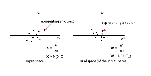
Figure 2 | an Axample when dimension = 2
We use the notation
${\bf X} = \begin{bmatrix} {\bf x_1} \\ \vdots \\ {\bf x_n} \end{bmatrix} $
to represent the random vector of input stimuli in the input space, $ {\bf W} = \begin{bmatrix} {\bf w_1} \\ \vdots \\ {\bf w_n} \end{bmatrix} $ to represent the random vector of neurons in the dual space. (Bold notation here means random variable)
(Relationship of input space and its dual space) Given a neuron represented as $ \left[ \begin{array}{c} w_1 \\ \vdots \\ w_n \end{array} \right] $, then this neuron’s tuning curve in the input space is $ n(x_1, … x_n) = w_1 x_1 + … + w_n x_n $, i.e., $ w_i = \frac{\partial n}{\partial x_i} $
The optimization problem now is to find the Gaussian distribution that has the sharpest discrimination, with the firing rate range being constrained.
Here both the gaussian distribution in the input space and the dual space is center at 0, so their distribution are only determined by the covariance matrix $ C, C_w $ respectively (Figure 2), where $ C = E({\bf XX^T}) $, $ C_w = E({\bf WW^T}) $.
The firing rate constraint is that the variance of the firing rate across neurons equals to a constant: $Var({\bf XW})=E({\bf XWW^T X^T}) = constant$
The objective function is $ det(C_w) $, intuitively this term describes how wide the gaussian distribution is (proportional to the volume of 95% confidence region, for example)
In summary, the optimization problem for efficient coding in this senario can be written as:
Given C, maximizing $det(C_w)$ with the constraint that $Var(XW) = a >0 $ (a is a constant).
We can derive the solution for this problem: \begin{equation} C_{w_{opt}} = \frac{a}{n} \bigotimes C^{-1} \end{equation}
$\bigotimes$ is the notation for multiplying every element of the matrix ($C^{-1}$) by a number ($\frac{a}{n}$). The details of the proof is at the end.
Biological meaning
We can be apply this solution to experiments.
Here is a simple example of a two dimensional senario. In experiment, an animal needs to view a sequence of images. The images are in a high dimensional space, but we only care about two of them. 1) How bright the images are, and 2) How large the images are. Thus, the pictures lay in a two-dimensional space one corresponding to the brightness of the image and the other corresponding to the size. Experimenters record neurons in a certain brain area, trying to find whether there are neurons responding to either of the dimension. Some neurons only respond to the brightness of the images, while some only respond to the size of the images, some neurons respond to both or neither. If the brightness and the size of the images are correlated, for example, images that are bigger also tend to be brighter. In order to best discriminate the brightness from size, how should the neurons as a population tuning to these two dimension?
This question can be converted to the optimization problem that we stated above. Equation (1) predicts that if the brightness and the size of the images are positively correlated, then neurons that respond positively to brightness should tend to negatively respond to the size, and vice versa.
In one experiment4, the authors have found that locally the neuron’s covariance matrix is roughly the inverse of the task variables covariance matrix, and this leads to “whitening operation”, which optimize the mutual information.
Proof of the optimization problem’s solution:
Firstly Let’s consider a simple case: Given $ C $ as an Identity matrix $ C = Id $, we want to find out the optimal solution of $C_{w} $, noted as $ C_{w_{opt}} $.
$ C$ is an Identity matrix, \(E(\mathbf{x_i x_j}) = \begin{cases} 0, & \text{if } i \ne j \\ 1, & \text{if } i = j \end{cases}\)
The constraint function can be written as:
\(\begin{aligned}
& a = Var({\bf XW}) = E({\bf X W W^T X^T}) \\
& = E({\bf X} C_w {\bf X}) \text{ , (} {\bf W} \text{ and } {\bf X} \text{ are independent)}\\
& = \sum_{i} E(C_w(i, i)), C \text{ is an identity matrix}\\
& = tr(C_w)
\end{aligned}\)
For objective function:
$ C_w $ is a positive definite matrix, so it has $n$ positive eigen values:
$ \sigma_1^2, \sigma_2^2,…, \sigma_n^2 $
And $ det(C_w) = \sigma_1^2 * \sigma_2^2 * … * \sigma_n^2 $
from the constraint condition we know:
$ \sigma_1^2 + \sigma_2^2 + … + \sigma_n^2 = tr(C_w) = a $
By the Arithmetic Mean-Geometric Mean inequality we can get $ det(C_w) = \sigma_1^2 * \sigma_2^2 * … * \sigma_n^2 <= (a/n)^n $ , and the equality is reached when $ \sigma_1^2 = \sigma_2^2 = … = \sigma_n^2 = \frac{a}{n} $
\(\Rightarrow
C_{w_{opt}} =
\begin{bmatrix}
a/n & 0 & \dots & 0 \\
0 & a/n & \dots & 0 \\
\vdots & \vdots & \ddots & \vdots \\
0 & 0 & \dots & a/n
\end{bmatrix}
= \frac{a}{n} \bigotimes Id\)
Hence, in this simple case, $ C_{w_{opt}} = \frac{a}{n} \bigotimes C^{-1} $
Now let’s consider the general case.
The input vector with arbitrary Gaussian distribution is centered at 0, and the covariance matrix C can be an arbitary positive definit matrix.
We change the basis of the input space such that the covariance matrix becomes an identity matrix, then the general case can be transformed to the first case:
Denote $ A $ as the change of basis matrix, $ {\bf X} $ as the random vector under old basis, and $ {\bf X’}$ as the random vector under new coordinates
$ {\bf X} = A{\bf X’} $, where $ {\bf X’} \sim N(0, Id) $, $ C = E({\bf XX^T}) = E(A{\bf X’X’^T}A^T) = AA^T$
The dual space’s basis should change accordingly.5
Denote $ {\bf W } $ as the random vector under old dual basis, $ {\bf W’}$ as the random vector under new dual basis, we have the relation:
$ {\bf W} = (A^{-1})^T {\bf W’} $
In the new basis, the solution of the optimization problem is given in case 1, $ C’_ {W_{opt}} = E({\bf W’W’^T}) = \frac{a}{n} \bigotimes Id $. In the old basis the solution is written as:
\(\begin{aligned}
C_{w_{opt}} & = E({\bf WW^T}) = E((A^{-1})^T {\bf W' W'^T} (A^{-1}))\\
& = (A^{-1})^T (\frac{a}{n} \bigotimes Id) A^{-1}\\
& = \frac{a}{n} \bigotimes (A^{-1})^T A^{-1}\\
& = \frac{a}{n} \bigotimes (A A^T)^{-1}\\
& = \frac{a}{n} \bigotimes C^{-1}\\
\end{aligned}\)
Thus we have $ C_{w_{opt}} = \frac{a}{n} \bigotimes C^{-1} $
Open discussion:
We can consider a even more general efficient coding problem. The input space can be an arbitrary manifold X, and the input stimuli have a given probability distribution on the manifold with probability density function $ f_X $. A neuron’s tuning curve is a smooth function on the manifold. Each neuron’s tuning curve is drawn independently from a set of functions(function space) with a certain probability distribution on the function space. We want to know the probability distribution on this function space that can maximize certain objective function. For example, an objective function could be
\[E_{w \in W}(\int_X |dw| f_X d \sigma)\]Reference:
[1]. Barlow, H.B., 1961. Possible principles underlying the transformation of sensory messages. Sensory communication, 1(01).
[2]. Simoncelli, E.P. and Olshausen, B.A., 2001. Natural image statistics and neural representation. Annual review of neuroscience, 24(1), pp.1193-1216.
[3]. Park, I.M. and Pillow, J.W., 2017. Bayesian efficient coding. BioRxiv, p.178418.
[4]. Koay, S.A., Thiberge, S.Y., Brody, C.D. and Tank, D.W., 2019. Sequential and efficient neural-population coding of complex task information. bioRxiv, p.801654.
[5]. https://math.stackexchange.com/questions/950290/help-on-the-relationship-of-a-basis-and-a-dual-basis
[6]. https://en.wikipedia.org/wiki/Harmonic_map